My mom always said don't drive around happy hour unless you want to be stuck in traffic (smart lady!). However, for the purposes of city planning, supply chain coordination, and emergency service routing, there is value in a more granular forecast. For my cyber physical systems seminar, I applied deep learning to the task of traffic forecasting.

How do we build a model to predict traffic? Traffic forecasting sounds simple at first: take the last hour of speed readings and predict the next hour. The problem becomes much more interesting when those readings come from 8,600 sensors at the same time. A model needs to learn how traffic changes over time, but also how every sensor relates to the rest of the road network. Standard attention, like in the original Transformer, can model those relationships well, although comparing every sensor with every other sensor becomes very expensive very quickly.

For this project I implemented four spatial-temporal forecasting models from scratch in PyTorch and evaluated them on the LargeST traffic benchmark. The main goal was to understand the tradeoff between forecasting accuracy and scalability, specifically how EiFormer replaces quadratic self-attention with a much cheaper latent attention mechanism.

The four models were TSMixer, RPMixer, iTransformer, and EiFormer. They all accept the same input, 12 previous five-minute traffic readings from every sensor, and predict 3, 6, or 12 future readings. This corresponds to forecasting traffic 15 minutes, 30 minutes, or one hour into the future.

Preparing the Traffic Data

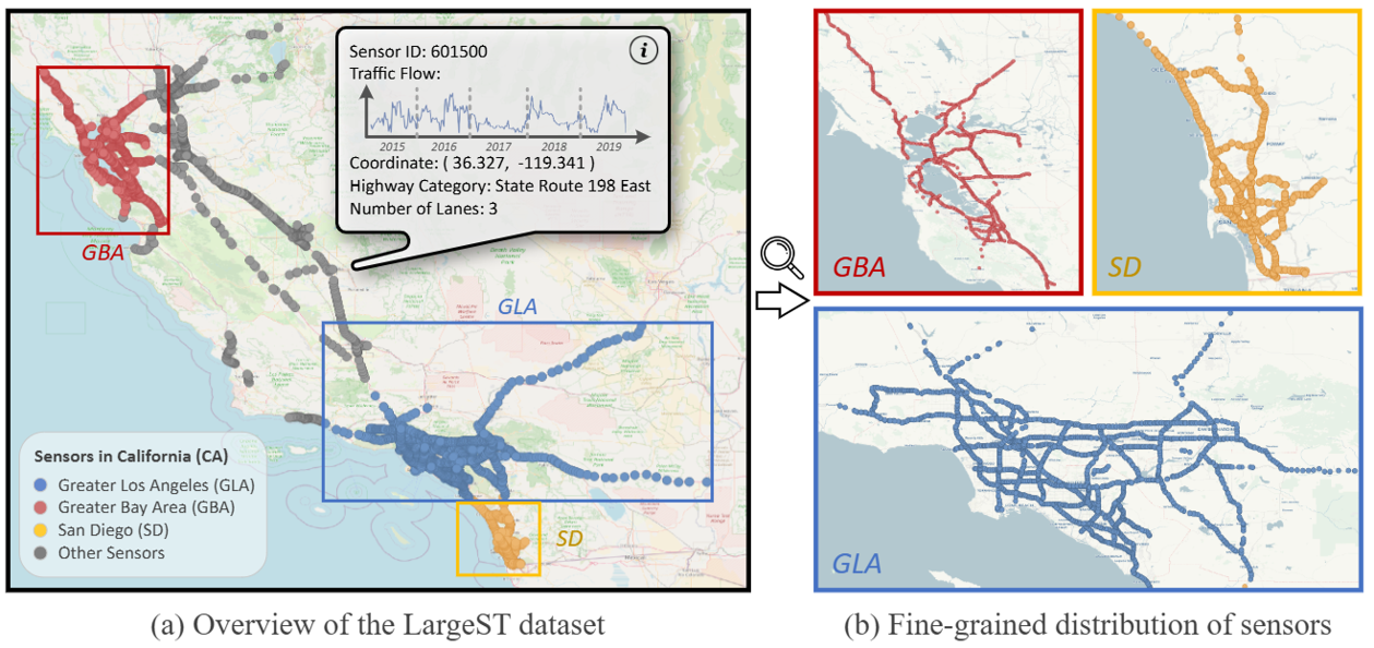
LargeST contains roughly 105,000 timesteps of California traffic speeds, divided into San Diego, the Greater Bay Area, Greater Los Angeles, and the entire state. The smallest split still has 716 sensors, while the full California dataset has 8,600.

I wrote a data pipeline that loads the HDF5 files, extracts the speed channel, replaces missing values with zero, and splits the data chronologically into 70% training, 10% validation, and 20% testing. It was important to split along the time axis instead of randomly, otherwise the model could train on future traffic and be evaluated on the past.

The normalizer is fit only on the training portion, then a sliding window turns the data into input and target pairs. The sliding window consists of 12 past readings from each of the sensors, fed into the model, which outputs a configurable number of future readings for each sensor.

Starting Without Attention

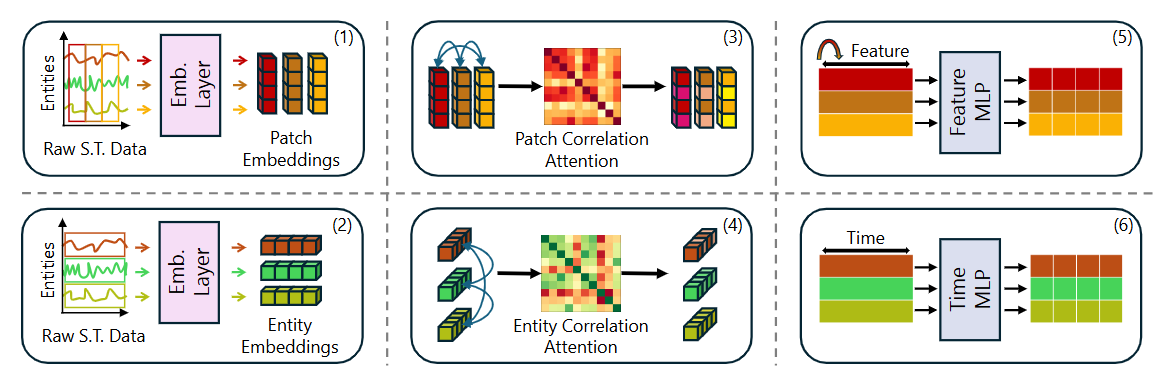
The first model I implemented was TSMixer, an architecture made entirely from MLPs. Each block first mixes the 12 values along the time axis independently for every sensor. A second MLP then mixes information across all sensors at each timestep. Both operations use residual connections, normalization, dropout, and a final temporal projection converts the history into the requested forecast length.

TSMixer is refreshingly simple and its computation grows roughly linearly with the number of sensors. However, the feature-mixing layer has a weight matrix built for one exact value of N. A model trained on San Diego's 716 sensors cannot be handed 717 sensors without rebuilding it.  

RPMixer uses the same mixer blocks, but first sends the inputs through a frozen random linear projection across sensors. The idea is that a fixed random view of the network can diversify the representations and act as a regularizer without adding more learned computation. Implementing this was mostly just creating a normal linear layer and disabling gradients for all of its parameters.

Turning Sensors into Tokens

iTransformer changes the usual interpretation of a transformer. Instead of treating each timestep as a token, it transposes the input and treats each sensor's entire history as one token. A linear layer embeds the 12 readings into a 64-dimensional vector, then multi-head attention learns relationships between sensors.

This approach has a nice property: none of its weights depend on the number of sensors. The same trained model can technically accept a different N at inference time. The downside is the attention map. For N sensors it contains N x N comparisons, so its memory and computation grow quadratically.

That isn't too concerning with San Diego's 716 sensors. With all 8,600 California sensors, one attention map contains almost 74 million relationships per example, per head. My experiment had to skip iTransformer on the full California dataset because it would exceed the available GPU memory.

Making Attention Linear

EiFormer keeps the useful inverted representation from iTransformer, but the keys and values no longer come from all N input sensors. Instead, each attention head has M latent keys and values, with M set to 16 in my experiments.

Q = embedded sensor histories                 (N x d)
scores = Q K^T / sqrt(d)                      (N x M)
attention = softmax(scores)
output = attention V                         (N x d)

This changes the attention map from N x N to N x M. Because M stays fixed as the road network grows, the attention cost is effectively linear in the number of sensors. For California that means comparing 8,600 sensors against 16 latent factors instead of against all 8,600 sensors.

The first EiFormer block uses randomly initialized keys stored as a frozen buffer. Later blocks learn their keys, while the latent values are learned in every block. Around this attention I added the same pieces expected from a transformer block: multiple heads, pre-layer normalization, residual connections, dropout, and a GELU feed-forward network.

One subtle implementation detail was making the frozen keys a registered buffer instead of a parameter with gradients disabled. This keeps them in the model's state dictionary and moves them to the GPU with the rest of the model, but prevents the optimizer from treating them like something it should update.

Running the Experiments

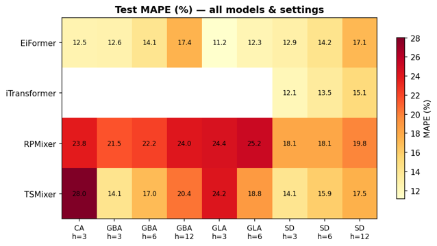
I set up one training interface for all four models and a SLURM array covering the combinations of model, region, and forecast horizon. Each run uses Huber loss, Adam, gradient clipping, a learning-rate scheduler, and early stopping based on validation MAE. Metrics are calculated after converting the predictions back to the original traffic-speed scale.

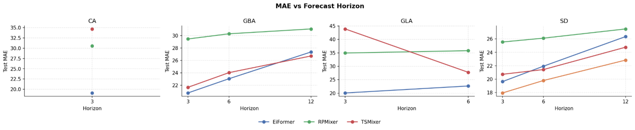
The completed results show the tradeoff pretty clearly. On the smaller San Diego dataset, full iTransformer attention produced the lowest MAE at every horizon: 17.93 at 15 minutes, 19.79 at 30 minutes, and 22.84 at one hour. Paying for every sensor-to-sensor comparison can be worthwhile when N is still manageable.

EiFormer became much more interesting as the network grew. It reached an MAE of 20.07 on the 3,834-sensor Los Angeles dataset for the 15-minute forecast, compared with 34.95 for RPMixer and 43.91 for TSMixer in these runs. Most importantly, it ran on all 8,600 California sensors with only 87,427 trainable parameters and reached a 15-minute MAE of 19.09. The mixer models used about 2.29 million parameters on the same dataset, while iTransformer could not reasonably run there with quadratic attention.

The results weren't a perfect sweep. TSMixer slightly beat EiFormer on the Bay Area one-hour forecast, and iTransformer remained strongest on the completed San Diego runs. I actually like this result more than a clean winner: latent attention is not automatically more accurate in every setting, but it makes transformer-style spatial modeling possible at a scale where full attention becomes impractical.

Remarks

In any DS&A class, there'll be some focus on the time complexity of algorithms. I don't believe that belief for searching for solutions < O(N^2) really sticks until you do a project with big data like this one, where O(N^2) changes which datasets the model can handle at all.

I gained a much better understanding of tensor shapes by implementing the architectures without relying on a forecasting library. Nearly every important operation is a transpose between (batch, history, sensors) and (batch, sensors, embedding). When one of those dimensions is wrong PyTorch will usually complain, but occasionally it will accept the shape and train something completely different, which is arguably more confusing.

Building a shared data loader, evaluation code, checkpointing, and cluster job array takes at least as much time (if not more) as implementing the attention equation. The model is the interesting part to talk about, but a fair comparison depends on all four models seeing the exact same experiment conditions. This project made it obvious that an idea and a model is only half the battle and that experiment design is an important skill to develop.