Microservices are convenient because they let us break a large system into smaller pieces that can be built and deployed independently. The tradeoff is that when something breaks, figuring out what actually happened becomes much harder. A request might pass through five different services before failing, and the service reporting the error isn't necessarily the one that caused it. As part of my machine learning course, I spent the semester researching a more efficient way to automatically detect these failures using metrics, logs, and distributed traces.

This project builds on MSTGAD, an existing graph-based anomaly detection model. I started by reproducing the results from the original paper. Then I replaced its most expensive temporal attention module with Mamba, a selective state space model that scales linearly with sequence length. I also experimented with detecting anomalies based on changes in the relationships between services. I called the final model MESTGAD: Mamba-Enhanced Spatial-Temporal Graph Anomaly Detection. Naming research models may be the easiest part of the process.

Turning Microservices into a Graph

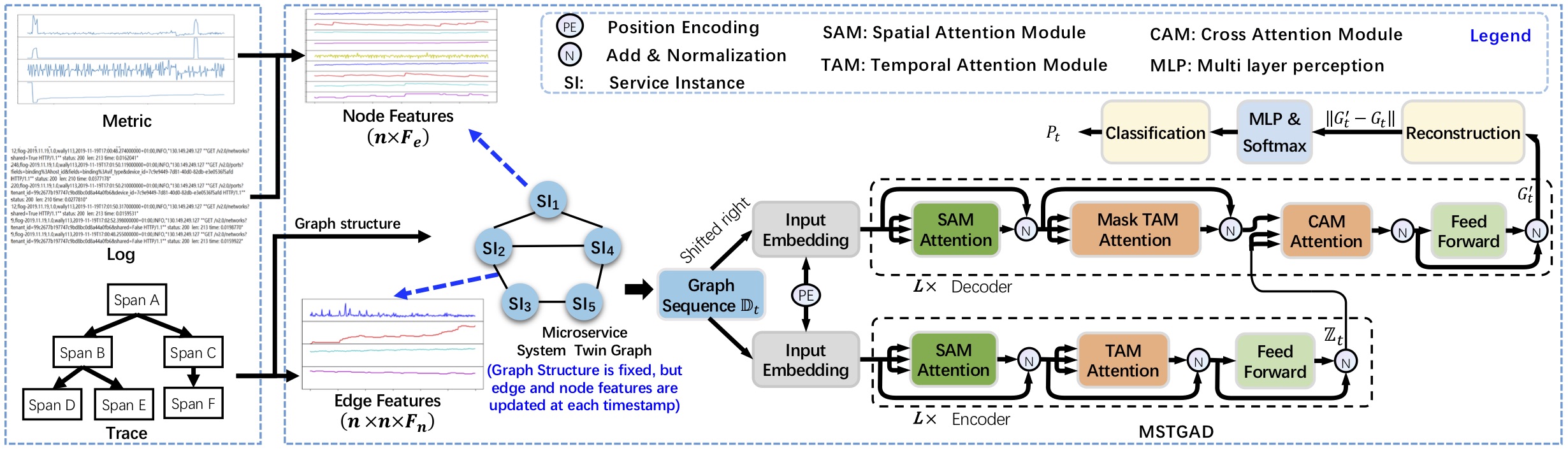
A microservice system already looks a lot like a graph. Each service or machine can be represented as a node, and requests traveling between services can be represented as edges. The more complicated problem is figuring out how to combine the three different types of data produced by the system.

Metrics like CPU utilization, memory usage, and network traffic become features on each node. Logs are parsed into templates, counted over time, and attached to the node that produced them. Distributed traces show how requests travel through the system, so the request type and duration become features on the edges. I normalize each input, align everything by timestamp, and divide the data into sliding windows. The result is a sequence of graphs describing the system over time.

MSTGAD uses spatial attention to decide which neighboring services and types of data are relevant to one another. For example, a latency spike is much more informative if the model can connect it to a burst of error logs and a slow trace between two particular services. This is the motivation for using a graph instead of training three unrelated anomaly detectors and hoping their outputs agree.

The Problem with Temporal Attention

The spatial attention handles relationships between services, but MSTGAD also uses temporal attention to compare different points within a sliding window. Standard attention compares every timestep with every other timestep. This means its time and memory complexity grow quadratically with the length of the window. Microservices add a spatial dimension on top of that, so increasing the number of services or the amount of history can make the model impractical pretty quickly.

Before changing the architecture, I reproduced MSTGAD on the MSDS dataset. MSDS contains metrics, log templates, and traces collected from five physical nodes in an OpenStack deployment. My reproduction reached an F1 score of 0.964 +/- 0.008, compared with 0.957 in the original paper. Establishing this baseline was important because without it, I wouldn't know if a later result came from my new architecture or from some difference in preprocessing, training, or evaluation.

Replacing Attention with Mamba

The main change in MESTGAD is replacing temporal attention in both the encoder and decoder with Mamba blocks. Instead of creating a matrix containing the relationship between every pair of timesteps, Mamba carries a hidden state forward through the sequence. Its parameters depend on the current input, which gives it the ability to remember useful information and ignore noise. The important part for this project is that its computation grows linearly with the window length instead of quadratically.

In my implementation, the node metrics, trace features, and log features each pass through their own Mamba block. I mix the node and log representations because both share the service axis, while the trace features continue along the graph edges. I designed the output tensor to have the same shape as the temporal attention module it replaced. As a result, I didn't have to redesign the spatial attention, cross-attention, decoder, or reconstruction portions of MSTGAD.

The decoder also has to be causal, meaning it can't cheat by looking at future data while reconstructing the current window. Attention enforces this with a mask. Mamba's recurrence only depends on the current and previous hidden states, so it is causal as a consequence of how the model works rather than because of an additional mask.

The interesting result was efficiency, not a dramatic improvement in accuracy. At window sizes of 10, 20, and 40, MESTGAD stayed within a few thousandths of the original model's F1 score. At window sizes of 80 and 160, MSTGAD ran out of memory on an NVIDIA L40S with 48 GB of memory. MESTGAD completed both experiments with F1 scores of 0.948 +/- 0.004 and 0.958 +/- 0.002. When I profiled the temporal modules by themselves, attention followed the expected quadratic growth while Mamba followed linear growth.

Looking for Changes Between Services

I also experimented with an anomaly signal called association discrepancy. Reconstruction error is good at detecting when an individual CPU metric, log count, or trace duration looks abnormal. However, a cascading failure might first show up as a change in how services interact. One service could suddenly depend much more heavily on another without either service immediately producing an extreme value.

The spatial graph-attention module already calculates weights representing the importance of service-to-service relationships. I compared those observed weights with a learned prior representing normal behavior using KL divergence. A large difference becomes another anomaly signal, which I combined with reconstruction error during inference:

anomaly score = reconstruction error + lambda * association discrepancy

This experiment produced what I would call a useful negative result. I swept lambda from 0 to 1, but the F1 score was basically flat. The best runs reached around 0.957, and their variance overlapped the result with association discrepancy turned off. My best explanation is that the anomalies in MSDS are mostly large changes in metrics and logs, which reconstruction error already detects. The relationship-based score may be measuring something real, but it doesn't add much new information for this particular dataset.

Training and Evaluation

MSDS has roughly 80 normal samples for every abnormal sample. Accuracy isn't very meaningful with that imbalance because a model could label almost everything as normal and still appear successful. I followed the semi-supervised setup from the original paper with a 60/10/30 training, validation, and test split, leaving half of the training labels unknown. The training objective combines graph reconstruction loss with cross-entropy classification. I evaluated the models using precision, recall, F1, AUC, and average precision instead of relying on accuracy alone.

I repeated every experiment across three random seeds. The full set of experiments included reproducing MSTGAD, sweeping the association-discrepancy weight, and testing both architectures across different temporal window sizes. Everything ran on a single NVIDIA L40S provided by the Holland Computing Center at the University of Nebraska-Lincoln.

Remarks

There is still more I would like to explore. MSDS only contains five service instances, so it doesn't really test the spatial scale that motivates the model. My next step would be evaluating MESTGAD on the larger AIOps-Challenge dataset or a synthetic system with many more services. I would also like to calculate association discrepancy from edge attention or incorporate it into training instead of adding it only during inference. It didn't improve F1 in the first version, but I still think it is an interesting way to catch failures that change the relationships inside a system before causing an obvious spike in a single metric.